Example

# NBVAL_IGNORE_OUTPUT
%load_ext watermark
import qutip
import numpy as np
from numpy import pi
import matplotlib
import matplotlib.pylab as plt
import newtonprop
%watermark -v --iversions

qutip       4.3.1
numpy       1.15.4
matplotlib  3.0.2
matplotlib.pylab  1.15.4
newtonprop  0.1.0
CPython 3.6.7
IPython 7.2.0

QuTiP Model

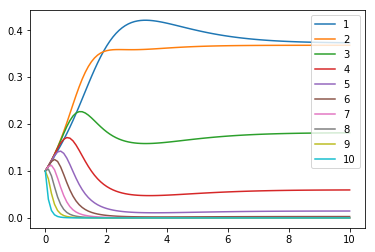
We consider the example of a driven harmonic oscillator with spontaneous decay, truncated to 10-levels. The dynamics start from the totally mixed state.

def liouvillian(N=10):

    two_pi = 2.0 * pi
    w_c = two_pi * 0.01
    gamma = two_pi * 0.1
    E0 = 0.5

    # Drift Hamiltonian
    H0 = np.array(np.zeros(shape=(N, N), dtype=np.complex128))
    for i in range(N):
        H0[i, i] = i * w_c

    # Control Hamiltonian
    H1 = np.array(np.zeros(shape=(N, N), dtype=np.complex128))
    for i in range(1, N):
        H1[i-1, i] = np.sqrt(float(i))
        H1[i, i-1] = H1[i-1, i]

    # Total Hamiltonian
    H = H0 + E0 * H1

    # Dissipator
    a = np.array(np.zeros(shape=(N, N), dtype=np.complex128))
    for i in range(1, N):
        a[i-1, i] = np.sqrt(i)

    a_dag = a.conj().T

    return qutip.Qobj(H), [qutip.Qobj(a), ]

def rho_mixed(N=10):
    rho = np.matrix(np.zeros(shape=(N, N), dtype=np.complex128))
    rho[:, :] = 1.0 / float(N)
    return qutip.Qobj(rho)

H, c_ops = liouvillian()

rho0 = rho_mixed()

L = qutip.liouvillian(H, c_ops)

tlist = np.linspace(0, 10, 100)

Reference Dynamics

We can use QuTiP’s mesolve routine to analyze the system dynamics:

result_mesolve = qutip.mesolve(L, rho0, tlist)

def plot_pop_dynamcis(result):
    data = np.array([state.diag() for state in result.states])
    fig, ax = plt.subplots()
    n = data.shape[1]
    for level in range(n):
        ax.plot(result.times, np.real(data[:, level]), label="%d" % (level+1))
    ax.legend()
    plt.show(fig)

plot_pop_dynamcis(result_mesolve)

For comparison with the Newton propagator which is supposed to be exect to a pre-specified limit (\(10^{-12}\), by default), it is better if we can compare to the propagation that results from exactly exponentiating the Liouvillian.

class Result():
    """Dummy class for propagation result"""
    pass

def propagate_expm(L, rho0, tlist):
    result = Result()
    result.times = tlist
    dt = tlist[1] - tlist[0]
    states = [rho0, ]
    rho = rho0
    E = (L * dt).expm()
    for _ in range(len(tlist)-1):
        rho = E(rho)
        states.append(rho)
    result.states = states
    return result

result_expm = propagate_expm(L, rho0, tlist)

def error(result1, result2):
    err = np.linalg.norm(
          result1.states[-1].full()
        - result2.states[-1].full())
    print("%.1e" % err)

This is our “exact baseline”. The mesolve routine is only exact to about \(10^{-7}\).

error(result_mesolve, result_expm)

1.2e-07

Newton propagation of QuTiP objects

First, we use the Newton propagator to simulate the dynamics using QuTiP objects.

def zero_qutip(v):
    return qutip.Qobj(np.zeros(shape=v.shape))

def norm_qutip(v):
    return v.norm("fro")

def inner_qutip(a, b):
    return complex((a.dag() * b).tr())

def propagate(L, rho0, tlist, zero, norm, inner, tol=1e-12):
    result = Result()
    result.times = tlist
    dt = tlist[1] - tlist[0]
    states = [rho0]
    rho = rho0
    for _ in range(len(tlist) - 1):
        rho = newtonprop.newton(
            L, rho, dt, func='exp', zero=zero, norm=norm, inner=inner, tol=tol
        )
        states.append(rho)
    result.states = states
    return result

Using the Frobenious norm here is absolutely critical: QuTiP’s default norm is not compatible with the inner product, and will lead to a subtle error.

result_qutip = propagate(
    L, rho0, tlist, zero_qutip, norm_qutip, inner_qutip, tol=1e-12
)

error(result_qutip, result_expm)

8.7e-11

result_qutip = propagate(
    L, rho0, tlist, zero_qutip, norm_qutip, inner_qutip, tol=1e-8
)

error(result_qutip, result_expm)

1.3e-09

Newton propagation of QuTiP objects with Cython

from qutip.cy.spmatfuncs import cy_ode_rhs
from qutip.superoperator import mat2vec

L_data = L.data.data
L_indices = L.data.indices
L_indptr = L.data.indptr
rho0_data = mat2vec(rho0.full()).ravel('F')

def zero_vectorized(v):
    return np.zeros(shape=v.shape, dtype=v.dtype)

def norm_vectorized(v):
    return np.linalg.norm(v)

def inner_vectorized(a, b):
    return np.vdot(a, b)

def apply_cythonized_L(rho_data):
    return cy_ode_rhs(0, rho_data, L_data, L_indices, L_indptr)

result_qutip_cython = propagate(
    apply_cythonized_L,
    rho0_data,
    tlist,
    zero_vectorized,
    norm_vectorized,
    inner_vectorized,
)

N = rho0.shape[0]
result_qutip_cython.states = [
    qutip.Qobj(rho.reshape((N, N), order="F"))
    for rho in result_qutip_cython.states
]

error(result_qutip_cython, result_expm)

3.5e-11

Using a stateful propagator

We can achieve exactly the same using the a stateful propagator class. While this seems a little more verbose at first, it allows for a much better abstraction:

class QutipNewtonPropagator(newtonprop.NewtonPropagatorBase):
    def _check(self):
        super()._check()
        if not isinstance(self._v0, qutip.Qobj) and self._v0.type == "oper":
            raise ValueError("v must be a density matrix")

    def _convert_state_to_internal(self, v):
        return mat2vec(v.full()).ravel("F")

    def _convert_state_from_internal(self, v):
        N = self._v0.shape[0]
        return qutip.Qobj(v.reshape((N, N), order="F"))

    def _inner(self, a, b):
        return np.vdot(a, b)

    def _norm(self, a):
        return np.linalg.norm(a)

    def _zero(self, a):
        return np.zeros(shape=a.shape, dtype=a.dtype)

    def _A(self, t):
        def A(rho_data):
            L = self._data
            return cy_ode_rhs(
                t, rho_data, L.data.data, L.data.indices, L.data.indptr
            )

        return A

def propagate_with_propagator(L, rho0, tlist, tol=1e-12):
    result = Result()
    result.times = tlist
    dt = tlist[1] - tlist[0]
    states = [rho0]
    propagator = QutipNewtonPropagator(L, tol=tol)
    propagator.set_initial_state(rho0)
    for time_index in range(len(tlist) - 1):
        t = tlist[time_index] + dt/2
        propagator.step(t, dt)
        states.append(propagator.state)
    result.states = states
    return result

result_qutip_propagator = propagate_with_propagator(L, rho0, tlist)

error(result_qutip_propagator, result_expm)

3.5e-11

Newton propagation of numpy state

Lastly, we consider the propagation using numpy objects only, by vectorizing the QuTiP objects:

def zero_vectorized(v):
    return np.zeros(shape=v.shape, dtype=v.dtype)

def norm_vectorized(v):
    return np.linalg.norm(v)

def inner_vectorized(a, b):
    return np.vdot(a, b)

rho0_vectorized = qutip.operator_to_vector(rho0).full().flatten()
Lmatrix = L.full()

def L_vectorized(v):
    return Lmatrix @ v

result_vectorized = propagate(
    L_vectorized,
    rho0_vectorized,
    tlist,
    zero_vectorized,
    norm_vectorized,
    inner_vectorized,
)

N = rho0.shape[0]
result_vectorized.states = [
    qutip.Qobj(rho.reshape((N,N), order='F'))
    for rho in result_vectorized.states]

error(result_vectorized, result_expm)

3.5e-11